Here's a bit more armchair audio. Prediction programs show us the spatial distribution of the magnitude of the sound pressure, which, generally, is what we want to know.
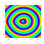
I got curious about how contours of constant phase might look. The possible practical value of this might be to find ways to arrange speakers so that non-collocated mains and subs might better combine over a larger listening area. (I know, this is probably a fool's errand, but it's what got me interested.)
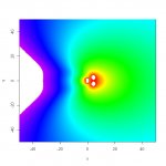
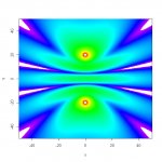
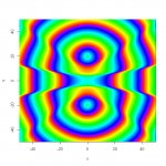
So I wrote a VERY basic 2-D prediction program to have a look. The R code is included in its entirety below. The sources are all ideal point sources and there is no smoothing in space or frequency. The example images are for a typical end-fire sub array at the null frequency of 62.5 Hz, and for a split mono system, also at 62.5 Hz, with the sources separated by 40 ft.
Interesting to me are the phase discontinuities at the nulls in the pattern for the split case.
It would be cool, if not useful, for commercial prediction programs to let us see phase. The information is already computed -- it just needs to be displayed. (Danley/GPA??)
Reinventing the wheel, as always,
--Frank
---------------------------------------------------------------------------------------
rm(list = ls())
X <- 100 #length of prediction (ft)
Y <- 100 #width of prediction (ft)
res <- 4 #spatial resolution (points/ft)
M <- X * res
N <- Y * res
x <- (1:M - M/2) / res
y <- (1:N - N/2) / res
f <- 62.5 #frequency (Hz)
omega <- 2 * pi * f #frequency (rad/s)
c <- 1130 #velocity (ft/s)
k <- omega / c #wave number (1/ft)
I <- 4 #number of sources used in this run
S <- matrix(nrow = 10, ncol = 4) #source parameters -- max of 10 sources allocated
S[1,1] <- 4.52 #x coord (ft)
S[1,2] <- 3 #y coord (ft)
S[1,3] <- 1 #sound pressure (relative)
S[1,4] <- .004 #delay (s)
S[2,1] <- 0
S[2,2] <- 1
S[2,3] <- 1
S[2,4] <- 0
S[3,1] <- 0
S[3,2] <- -1
S[3,3] <- 1
S[3,4] <- 0
S[4,1] <- 4.52
S[4,2] <- -3
S[4,3] <- 1
S[4,4] <- .004
d <- matrix(nrow = M, ncol = N) #distance to source at each point(ft)
p <- matrix(data = complex(1, 0, 0), nrow = M, ncol = N) #complex sound pressure at each point
for (i in 1:I){ #for each source
for (m in 1:M){ #for each x value
d[m, 1:N] <- ((x[m] - S[i,1])^2 + (y[1:N] - S[i, 2])^2)^.5
p[m, 1:N] <- p[m, 1:N] + complex(1, modulus = S[i,3] / d[m, 1:N], argument = k * d[m, 1:N] + S[i,4] * omega)
}
}
windows(7, 7) #plot magnitude
image(x, y, -20*log(Mod(p), 10), zlim = c(0, 42), col = rainbow(256, start = 0, end = .8))
windows(7, 7) #plot phase
image(x, y, Arg(p), zlim = c(-pi, pi), col = rainbow(256, start = 0, end = .8))
I got curious about how contours of constant phase might look. The possible practical value of this might be to find ways to arrange speakers so that non-collocated mains and subs might better combine over a larger listening area. (I know, this is probably a fool's errand, but it's what got me interested.)
So I wrote a VERY basic 2-D prediction program to have a look. The R code is included in its entirety below. The sources are all ideal point sources and there is no smoothing in space or frequency. The example images are for a typical end-fire sub array at the null frequency of 62.5 Hz, and for a split mono system, also at 62.5 Hz, with the sources separated by 40 ft.
Interesting to me are the phase discontinuities at the nulls in the pattern for the split case.
It would be cool, if not useful, for commercial prediction programs to let us see phase. The information is already computed -- it just needs to be displayed. (Danley/GPA??)


Reinventing the wheel, as always,
--Frank
---------------------------------------------------------------------------------------
rm(list = ls())
X <- 100 #length of prediction (ft)
Y <- 100 #width of prediction (ft)
res <- 4 #spatial resolution (points/ft)
M <- X * res
N <- Y * res
x <- (1:M - M/2) / res
y <- (1:N - N/2) / res
f <- 62.5 #frequency (Hz)
omega <- 2 * pi * f #frequency (rad/s)
c <- 1130 #velocity (ft/s)
k <- omega / c #wave number (1/ft)
I <- 4 #number of sources used in this run
S <- matrix(nrow = 10, ncol = 4) #source parameters -- max of 10 sources allocated
S[1,1] <- 4.52 #x coord (ft)
S[1,2] <- 3 #y coord (ft)
S[1,3] <- 1 #sound pressure (relative)
S[1,4] <- .004 #delay (s)
S[2,1] <- 0
S[2,2] <- 1
S[2,3] <- 1
S[2,4] <- 0
S[3,1] <- 0
S[3,2] <- -1
S[3,3] <- 1
S[3,4] <- 0
S[4,1] <- 4.52
S[4,2] <- -3
S[4,3] <- 1
S[4,4] <- .004
d <- matrix(nrow = M, ncol = N) #distance to source at each point(ft)
p <- matrix(data = complex(1, 0, 0), nrow = M, ncol = N) #complex sound pressure at each point
for (i in 1:I){ #for each source
for (m in 1:M){ #for each x value
d[m, 1:N] <- ((x[m] - S[i,1])^2 + (y[1:N] - S[i, 2])^2)^.5
p[m, 1:N] <- p[m, 1:N] + complex(1, modulus = S[i,3] / d[m, 1:N], argument = k * d[m, 1:N] + S[i,4] * omega)
}
}
windows(7, 7) #plot magnitude
image(x, y, -20*log(Mod(p), 10), zlim = c(0, 42), col = rainbow(256, start = 0, end = .8))
windows(7, 7) #plot phase
image(x, y, Arg(p), zlim = c(-pi, pi), col = rainbow(256, start = 0, end = .8))
